AI for Medical Diagnosis - Concepts

Coursera & deeplearning.ai – AI for Medicine Specialization

Course 1 – AI for Medical Diagnosis

The chest X-ray is one of the most common diagnostic imaging procedures in medicine with ~ 2 billion chest X-rays taken a year. Chest X-ray interpretation is critical for detecting pneumonia, lung cancer, etc.

An abonormality in chest X-rays is called a mass. A mass is defined as a lision or damaged tissue seen on a chest X-ray as greater than 3cm in diameter.

During training, an algorithm is shown images of chest X-rays labeled with whether they contain a mass or not. The algorithm learns using these images and labels and it produces an output of whether the X-ray contains a mass. The algorithm can be a:

• Deep Learning algorithm
• Model
• Convolutional Neural Network

The algorithm produces an output in terms of scores which are probabilities that the image contains a mass.

Key Challenges for Training Algorithms on Medical Images

1. Class Imbalance
2. Multi-Task
3. Dataset Size

Class Imbalance

There is not an equal number of examples of non-disease (normal) and disease (mass) in medical datasets. This is a reflection of the prevalence or the frequency of disease in the real-world where we see that there are far more examples of normals than of mass, especially when looking at X-rays of a healthy population. In a medical dataset, we might see 100 times as many normal examples as mass examples. This creates a problem for the algorithm which would see mostly normal examples. This yields a model that starts to predict a very low probability of disease for everybody and won’t be able to identify an example that has a disease.

Let’s say we have 8 images, 6 of which are normal and 2 are mass. The value of the loss function is 0.3 for each.

Total Loss from Mass Examples = 0.3 * 2 = 0.6

Total Loss from Normal Examples = 0.3 * 6 = 1.8

Most of the contribution to the loss comes from normal examples rather than from the mass examples, so the algorithm is optimizing its updates to get the normal examples right and it is not giving much relative weight to the mass examples. This will not produce a very good image classifier. This is a class imbalance problem.

The solution to this problem is to modify the loss function to weigh the normal and the mass classes differently. We can assign weights to the positive and negative examples. \(W_{p}\) for positive and \(W_{n}\) for negative. In this case, we want to weigh the mass examples more so they can have en equal contribution overall to the loss as the normal examples. Let’s select 6/8 as the weight for the mass examples and 2/8 as the weight for the normal examples.

\(W_{p}\) or \(W_{n} *\) \(loss\)

\(W_{n} = 2/8 * 0.3\) \(= 0.075\)

\(W_{p} = 6/8 * 0.3\) \(= 0.225\)

Total Loss from Mass Examples \(= 0.225 * 2 = 0.45\)

Total Loss from Normal Examples \(= 0.075 * 6 = 0.45\)

As we can see, if we sum up the total loss from the mass example we get 0.45 and this is equal to the total loss of the normal examples. In general, the weight we would put on the positive class will be the number of negative examples over the total number of examples.

\(W_{p} = num negative / num total = 6/8\) (6 normal examples / 8 (total) examples)

\(W_{n} = num positive / num total = 2/8\) (2 positive cases / 8 (total) cases)

So now, the positive and negative class contributions to the loss are the same. This is the idea of modifying the loss using weights and this method is called the Weighted Loss which is used to tackle the class imbalance problem.

Weighted Loss Equation

• The loss is made up of two terms:
  • \(loss_{pos}\): we’ll use this to refer to the loss where the actual label is positive (the positive examples).
  • \(loss_{neg}\): we’ll use this to refer to the loss where the actual label is negative (the negative examples).
• Note that within the \(log()\) function, we’ll add a tiny positive value, to avoid an error if taking the log of zero.

\[loss^{(i)} = loss_{pos}^{(i)} + los_{neg}^{(i)}\] \[loss_{pos}^{(i)} = -1 \times weight_{pos}^{(i)} \times y^{(i)} \times log(\hat{y}^{(i)} + \epsilon)\] \[loss_{neg}^{(i)} = -1 \times weight_{neg}^{(i)} \times (1- y^{(i)}) \times log(1 - \hat{y}^{(i)} + \epsilon)\] \[\epsilon = \text{a tiny positive number}\]

Re-sampling

We can also fix the class imbalance problem by re-sampling. The idea here is to re-sample the dataset to have an equal number of normal and mass examples.

To achieve this:

• Group the Normal and Mass examples together
• From these two groups, sample the images so that there is an equal number of positive and negative samples. This can be done by sampling half of the examples from the mass class and half of the examples from the normal class. Keep in ming that we will not be able to include all of the normal samples when re-sampling and – we might have more than one copy of the mass examples in the re-sampled dataset. If we compute the loss function without the weights (the regular binary cross-entropy loss) we will see that there is an equal contribution to the loss from the mass and normal examples.

There are many variations of this approach, we can under-sample the normal class and over-sample the mass class.

Multi-task Challenge

Thus far we have been talking about binary classification – identifying the samples as mass or not mass. In the real world we care about classifying the presence or absence of many diseases such as:

• Mass or No Mass
• Pneumonia or No Pneumonia
• Edema or No Edema

One way to attempt to solve these problems would be to have models that would learn each of these tasks. But it is also possible to do all these taks using one model. The advantage being that the model can learn features that are common to identifying more than one disease therefore we can use the data more efficiently. This set-up is caled Multi-task Learning. We can train an algorithm to learn all of these taks at the same time. In this learning environment, the examples would contain more information in their labels so instead of having info just about mass– the label can also contain info about other diseases such as pneumonia and edema. For instance (and for mass, pneumonia, and edema):

P1 0, 1 ,0

P2 0, 0, 1

P1 would indicate the absence of mass, the presence of pneumonia and the absence of edema.

P2 would indicate the absence of mass, the absence of pneumonia and the presence of edema.

Edema excess fluid in the lungs.

Also, instead of having one single output as we saw before now we have three different outputs denoting the probability of the three different deseases.

Prediction Probabilities

P1 0.3, 0.1, 0.8

P1 0.1, 0.1, 0.8

To train such an algorithm, we need to make a modification to the loss function from the binary task to the multitask setting.

We need to modify the loss function so it can look at the error associated with each disease.

\[L(X,y_{mass}) + L(X,y_{pneumonia}) + L(X,y_{edema})\]

We can then represent the new loss function as the sum of the losses over the multiple diseases:

\(L(X,y)\) \(MultiLabel / MultiTask \\ Loss\)

Loss

P1 0.52 + 1.00 + 0.70

P2 0.05 + 0.05 + 0.10

Class Imbalance can also be an issue in a multi-taks setting. But just as before, we can also apply the weighted loss to a multi-task.

\[MultiTask \quad L(X,y_{mass}) + L(X,y_{pneumonia}) + L(X,y_{edema})\] \[L(X, y_{class}) = \begin{cases} - W_{p, \ class}\ log P(Y = 1 | X) & \quad \text{if } y \text{ = 1}\\ - W_{n, \ class}\ log P(Y = 0 | X) & \quad \text{if } y \text{ = 0} \end{cases}\]

Here besides having the weights associated with the positive and negative labels we also have the associated class.

Dataset Size Challenge

For many medical imaging problems the architecture of choice is the Convolutional Neural Network (CovNet or CNN). These are designed to process 2D images such as X-rays. But variants of these are also used for medical signal processing or 3D medical images such CT scans. Several CNN architectures such as Inception, ResNet, DenseNet, ResNeXt and EfficientNets are very popular in the image classification field. In the medical field, the standard is to try out multiple models on the task at hand and evaluate which works best.

All these architectures consume and require lots of data and benefit from examples found in image classification datasets.

• General purpose images – millions of images with labels
• Medical image datasets – typically have 10K to 100K samples.

Medical image datasets do not have the luxury of having millions of examples which creates challenges. One solution is to pre-train the network. Have it look at natural images and learn how to identify different objects (cats, dogs, etc.), then use it as a starting point in a medical imaging task by transfering learned features. The network can then be further trained using chest X-rays to identify the presence or absence of diseases. In simply terms, having the network train on general images allows it to learn general features that can then help it learn on medical tasks. For instance, the features that it learned when identifying the shape of a penguin can be used to identify the edges of a lung. When we transfer these learned features to a new network, it can then learn how to interpret an X-ray with a better starting point. The first step of the process is called Pretraining and the second is called Fine-tuning

It is generally understood that the early layers of the network capture low-level image features that can be broadly generalized while the later layers capture features that are more high-level or more specific to a task. So, early layers might learn about the edges of an object (penguin) which can be later used for X-ray interpretation. When fine-tuning the layers of the network on X-rays instead of doing it on all features that were transferred, we can freeze the features learned by the shallow layers and just fine-tune the deeper layers.

In practice, we have two design choices:

1. Fine-tune all of the layers
2. Only fine-tune the later or last layer and skip the earlier layers

This fine-tuning approach is also called Transfer Learning and it help us solve the small dataset challenge.

Another approach to solving the dataset size challenge is tricking the network into thinking we have more data that we actually do. Right before we pass an image to the network we can apply a transformation to it. We have several options to do this:

• Rotate the image and pass it in
• Translate sideways and pass it in
• Zoom in
• Change brightness or contrast
• Apply a combination of these transformations

These methods are called Data Augmentation

In practice, there are two questions that drive the choice of transformations we pick.

1. Do augmentations reflect variations in the real world?
   • We can consider that there could be variations in contrast in natural X-rays, so we can have a transformation that chages the contrast of the image.
2. Do augmentations keep the label the same?
   • If we laterally invert the patients X-ray, (flipping left to right and right to left) then the heart would appear on the left-hand size of the image (the right of the body). In this case the label would no longer be valid because the image will now show a rare heart condition called dextrocardia in which the heart points to the right side of the chest instead of to the left side. This transformation would not preserve the label. The crucial point here is that we want the network to learn to recognize images with these transformations that still contain the same label.

Besides chest X-ray images there are other images that can benefit from rotating and flipping such as those used in hystopathology algorithms that detect skin cancer.

Model Testing

When doing Machine Learning, we need to split a dataset into a:

• Training set
• Used for development of models
• Training set can be furter split into a:
  • Validation set - used for tuning and selection of models
• The split into training and validation can be done multiple times and it’s called Cross-Validation
• Test set
• Used for reporting results

There are also othe names used to refer to these sets:

Training set => “Development Set”

Validation set => “Tuning set” or “dev set”

Test set => “holdout set” or “validation set”

There are three challenges with building these sets in the context of medicine.

1. Relates to how we make these test sets independent
2. Relates to how we sample them
3. Relates to how we set the ground truth

Problem of Patient Overlap

A patient has come two different times to get X-rays. Both times wearing a necklace which is present in both X-ray images. One of the images is sampled as part of the training set and the other is sampled as part of the test set. We train the deep learning model and it correctly predicts the output in the test set. However, it is possible that the model actually memorized the output when it saw the image of the patient with the necklace on. This is not a hypothetical scenario as deep learning models can unintentionally memorize training data and the model could memorize rare or unique training data aspects such as the necklace in the image which helps them get the right answer when testing on the same patient. This would lead to a Over-optimistic Test set Performance where we would think that the model’s performance is better that it actually is.

To address this problem in our dataset, we can ensure that a patient’s X-rays only occur in one of the datasets. For instance, put both images (with the necklace) in the training set. Now the model can learn its features but it does not help it achieve higher performance on the test set because it does not see the same patient.

Splitting Data by Patient

When split the dataset, images are randomly placed into one of the sets. If a sigle patient has multiple X-rays they can appear in more than one or all sets. This is Patient Overlap. To avoid it, we can split the dataset by patient thus all the images belonging to a single patient would be in the same set.

Refer to Week 1 Lab to see how to solve this issue.

AI for Medical Diagnosis Lab 1 Notebook

Set Sampling Challenge

Often times the size of the test set is a fraction of the full dataset, let’s say ~10%. Some of these sets need to be annotated by human readers. This can create a bottleneck for the test set size as it depends on how many examples can readers be expected to read. The challenge with sampling a test set is that when it is being randomly sampled from hundreds of examples, we might not sample any patients that actually have a disease. If images that do not contain a mass are in the test set then there is no way to actually test the performance of the model on positive cases. This is a prevalent problem with medical data where the dataset might be small and with not that many examples of positive cases for each disease.

One way to address this problem, is to sample a test set so that we have, at least, \(x\) % of examples of a minority class which in this case would be images containing a mass or positive cases. One common choice of \(x\) is 50% so if we are sampling a test set of 100 examples half of them would be positive and 50 would be negative cases. This would ensure that we have sufficient numbers to test the performance of the model on both cases.

Once the test set is sampled then the validation test should be sampled next and before training occurs. We would want the validation set to reflect the distribution of the data so to sample it– the same strategy used for the test set should be employed.

Ground Truth / Reference Standard

The concept of a right label in Machine Learning is the Ground Truth and in Medicine is the Reference Standard.

Evaluating a chest X-ray can be a complex task. One expert can identify pneumonia whereas other can look at the same image and see something different. This is called inter-observer disagreement and it is common in medical settings. The challenge here is how to set the ground truth required for the evaluation of algorithms in the presence of inter-observer disagreement. We can address this challenge by using the Consensus Voting method which requires the use of human experts to determine the ground truth. For instance, we can have three radiologist look at the chest X-ray in question and each determine whether there is pneumonia present or not. If two out of the three say yes– then the answer is yes. Generally speaking, the answer would be the majority vote of the three radiologists. Alternatively, we can have the three radiologits discussed this in a room and reach a single decision which would then be considered the ground truth.

The second method would be to use a more definitive test which provides additional information to set the ground truth. For instance, to determine whether a patient has a mass using a chest X-ray, a more definitve test that can be performed is a CT scan. A CT scan would show a 3D image of the abnormality thus giving the radiologist more information to reach a determination. If the mass is confirmed by the CT then we can assign the ground thruth to the chest X-ray. In dermatology, the ground truth for the test set was determined by a skin lesion biopsy.

The issue with this method is that we might not have more definitive tests available as not everyone gets a chest X-ray and a CT scan.

Calculating the PPV in terms of Sensitivity, Specificity and Prevalence

Rewriting PPV

\(PPV = P(pos|\hat{pos})\) pos is actually “positive” and pos hat is “predicted positive”

By Bayes rule, this is:

\[PPV = \dfrac {P(\hat{pos}|pos * P(pos)}{P(\hat{pos})}\]

For the numerator:

\(Sensitivity = P(\hat{pos}|pos)\) Keep in mind that sensitivity is how well the model predicts actual positive cases as positive.

\(Prevalence = P(pos)\) Prevalence is how many actual positives there are in the population.

For the denominator:

\(P(\hat{pos})= TruePos+FalsePos\) The model’s positive prediction are the sum of it when it correctly predicts positive and incorrectly predicts positive.

The true positives can be written in terms of sensitivity and prevalence. \(TruePos = P(\hat{pos}|pos) * P(pos)\) We can use substitution to get: \(TruePos = Sensitivity * Prevalance\)

The false positives can also be written in terms of specificity and prevalence:

\(FalsePos = P(\hat{pos}|neg)*P(neg)\) \(1 - Specificity = P(\hat{pos}|neg\) \(1 - Prevalence = P(neg)\)

PPV Rewritten:

If substituting these into the equation we get:

\[PPV = \dfrac{Sensitivity * Prevalence}{Sensitivity * Prevalence+(1-Specificity)*(1-Prevalence)}\]

ROC Curve

The ROC curve is one of the most useful tools when evaluating medical models. The ROC curve allows us to plot the sensitivity of a model against the specificity of the model at different decision thresholds. When we evaluate a chest X-ray image using a model, the model provides an output which is the probability of disease of such image. This output can be transformed into a diagnosis using a threshold or operating point. When the probability is above the threshold then we interpret this as positive – the patient has a disease – but if the probability is below the threshold we interpret this as negative – the patient does not have a disease. For instance, if the probability is 0.7 and the threshold is 0.5 then we would interpret the image as positive. If the probability is 0.3 and the threshold is 0.5 then we would interpret the image as negative. Please note that the threshold affects the metrics we use to evaluate the model. Let’s say the threshold is 0 then every image would be interpret as postive so the Sensitivity would be 1 whereas the Specificity would be 0. Now let’s say the threshold is 1 then every image would be classified as negative. The Sensitivity would be 0 and the specificity would be 1.

Notes on AI for Medicine – Week 3

MRI Images

MRI images are not 2D images like X-rays, an MRI sequence is a 3D image that consists of multiple 3D volumes. We can think of these volumes/sequences as channels similar to RGB channels in a regular image. However, an MRI image can contain more than 3 channels. These channels get stacked in the depth dimension to create an MRI image. One challenge when combining sequences is that the images can be misaligned due to patients moving or tilting their heads when the scan is being performed. If the images are not aligned with each other when we combine them– the brain region at one location in one channel would not correspond to the same region of the brain in the other channels. To fix this problem we use a technique called image registration The idea behind Image Registration is to transform the images so that they are aligned or registered with each other. Once the images have been registered we are able to combine the different sequences. This technique can be applied to all the slices of the brain. Now that these data have been combined then we can turn to the task of segmentation

Brain Tumor Segmentation

Segmentation is the process of defining the boundaries of various tissues. In this case we are trying to define the boundaries of tumors. We can also think of segmentation as the task of determining the class of every point in the 3D volume. These points– in a 2D space are called pixels and in a 3D space are called voxels There are two approaches to segmentation with MRI data:

1. 2D Segmentation. In this approach we break the 3D MRI volume into many 2D slices. Each one of these slices is passed to the segmentation model which outputs the segmentation for that slice. One by one, each slice is passed to the segmentation model to generate the segmentation for each slice. These 2D slices can then again be combined to form a 3D output volume of the segmentation.
   • The drawback with this approach is that we can lose important 3D context. For instance, if there is a tumor in one slice, there is likely to be a tumor in the slices adjacent to it. Since we are passing in slices one at a time to the network, the network is not able to learn this useful context.
2. 3D Segmentation. In this approach, we would want to, ideally, pass the entire MRI volume into the segmentation model and get a 3D segmentation map of the whole MRI as output. However, due to the size of the entire MRI volume it makes it nearly impossible to pass it in all at once into the model. It would be too expensive computationally and memory-wise. To solve this issue we can break up the 3D MRI volume into many 3D sub volumes. Each of these sub volumes would have some width, height, and depth context. Like in the 2D approach, we can now feed these sub volumes one at the time to the model and then aggregate them at the end to form a segmentation map of the whole volume.
   • The disadvantage with this 3D approach is that we might still lose some spatial context. For instance, if there is a tumor in one sub volume, there is likely to be a tumor in the surrounding volumes too. Since we are passing sub volumes one at the time into the network, the network might not be able to learn from possibly useful context.
   • The advantage with this approach is that we are capturing some context in all of the width, height, and depth dimensions.

Segmentation Architectures

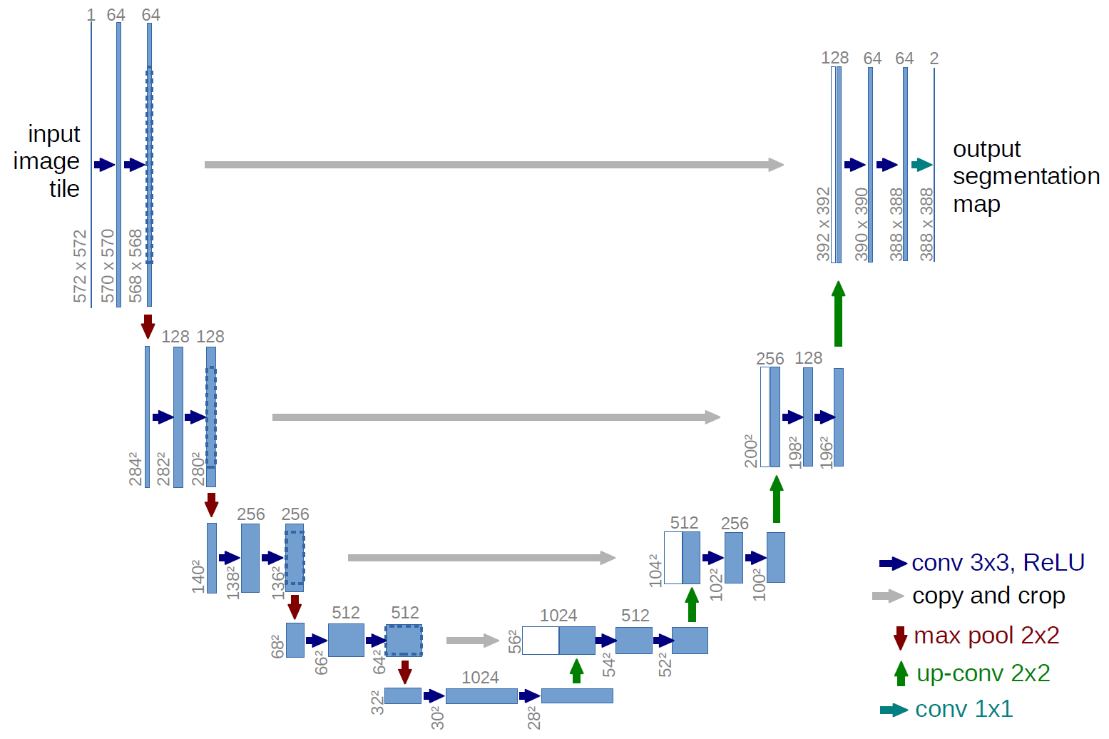
One of the most popular architectures for segmentation is U-Net which was first designed for biomedical image segmentation and has performed well in the task and cell tracking. U-Net can achieve good results even with only hundreds of examples. The U-Net architecture consists of two paths (starting at the top left side of the U):

1. Contracting path. This is a typical Convolutional Neural Network like the ones used in image classification. It consists of repeating applications of convolution and pooling operations. The convolution operation here is called down convolution. The key here is that in the contracting path the feature maps get spatially smaller which is why it is called a contraction
2. Expanding path. This path is doing the opposite of the contracting path as it takes the small feature maps through a series of up-sampling and up-convolution steps to get back to the original size of the image. It also concatenates the up-sample representations at each step with the corresponding feature maps at the contraction pathway. At the last step, the architecture outputs the probability of tumor for every pixel in the image. The U-Net architecture can be trained on input/output pairs of 2D slice if using the 2D approach. We can also use the 3D approach by replacing the 2D operations with their 3D counterparts. This is exactly what the 3D U-Net architecture does. The 2D convolutions become 3D convolutions and the 2D pooling layers become 3D pooling layers. 3D U-Net allows us to pass in 3D sub volumes and get an output for every voxel in the volume specifying the probability of a tumor.

For more info visit the U-Net creators’ site